Notes on Migrating a Linux Install

Some issues I ran into when trying to move a Linux install from a 500 GB drive to a smaller 120 G SSD:

• When duplicating the filesystem, make sure that /proc exists, otherwise when you boot the new drive the kernel will complaint that /proc is missing and it can't create the virtual file system
• In grub-rescue, (hd0,msdos2) is /dev/sda2, and (hd0,msdos1) is /dev/sda1
• When specifying initrd be sure not to accidentally select the vmlinuz image again
• After you have fixed grub and find that booting is taking longer than expected, check that the UUID in /etc/initramfs-tools/conf.d/resume is the UUID of your swap partition. Check using sudo blkid

Reading Lecroy Binary Waveform in Python

I needed to read Lecroy binary waveforms files recently, and the one python script I had found didn't read them properly due to improper handling of 16 bit samples.

I wrote an alternative lecroy.py that should be a drop-in replacement. It  handles 16 bit waveforms and exports a LecroyBinaryWaveform class that also provides additional metadata. It supports saving to CSV for binary to text conversion.

On the Use of I/Q Signals

• All signals are complex, that is they have the form of $$x(t)=A\exp(i\omega t)$$. I/Q presentation of a signal fully captures this by storing the real component in the I, the in-phase signal, and the complex component in Q, the quadrature signal.
• When we force signals to be purely real, e.g. $\cos(\omega t)$, we taking the real part of $exp(i\omega t)$. Because we ignore the imaginary component, we lose information. Specifically, $\cos(\omega t)$ can be the real part of $\exp(i\omega t)$ or $\exp(-i\omega t)$. We don't know any more.
• This ambiguity is present in the exponential form of $\cos$: $$\cos(\omega t) = \frac{\exp(i \omega t) + \exp(-i\omega t)}{2}$$. Note the presence of the two complex signals whose sum is always purely real as their imaginary parts cancel out. The real part of either complex signal will produce $\cos(\omega t)$.
• This ambiguity is why when you multiply $\cos(\omega_0 t)$ and $\cos(\omega_1 t)$ you end up with $\cos[(\omega_0 + \omega_1)t]$ and $\cos[(\omega_0 - \omega_1)t]$. In other words, the frequency add as $\pm \omega_0 \pm \omega_1$, which produces 4 unique combinations that reduces to 2 because $\cos$ is even.
• The result of multiplying real cosines produces two peaks in the frequency spectrum.
• On the other hand, preserving the complex nature of a signal by presenting it as $A\exp(i\omega t)$ means that multiplying two signals together produces a unique result: $$A_0\exp(i\omega_0 t) \times A_1\exp(i\omega_1 t) = A_0A_1\exp[i(\omega_0 + \omega_1)t]$$. This is because there is no ambiguity as we have not thrown away any information.
• The result of multiplying complex signals produces one peak in the frequency spectrum.
• This is one of the advantages of working with I/Q data, which preserves the complex nature of signals, and allows us to frequency shift a signal through multiplication without also generating an additional unwanted image of the signal.

Cheers,

Steve

Simple FM Receiver with GNU Radio and RTL-SDR

Introduction

I recently started playing around with software defined radio using a USB TV tuner dongle utilising the popular RTL2832U chipset. After playing around with software like CubicSDR and gqrx I was somewhat frustrated at the opaqueness of what is going on under the hood. As such I resolved to learn GNU Radio so I can do the signal processing myself. Starting with a basic FM receiver seems like a good idea, since one of my goals is to receive NOAA APT transmissions, which are FM modulated at 137 MHz.

The Radio

The image below is the FM radio (source code) I built in GNU Radio Companion. GNU Radio Companion is part of GNU Radio that makes it pretty easy to graphically put together a custom signal processing chain and "make" a radio in software. I am not usually a big fan of graphical programming, but in this particular instance I have to admit the going was a lot easier than if I had to do this textually. There is built in support for documenting each block, which is nice, though I wish I had more control over the font used and the size of the text boxes.

FM radio created in GNU Radio Companion.

It looks more complicated than it is. Basically, the output from the receiver, which is centred around the central frequency, is down-sampled from 2.4 MHz to 500 KHz, then low-pass filtered and then passed to a FM demodulator module. The output of the FM demodulator is then resampled to 48 KHz and piped to an audio sink, i.e. a sound card.

All the extra stuff is are GUI controls and visualisations to aid in understanding and debugging.

This is what it looks like running, tuned a local station at 99.1 MHz, which is BBC Radio 1.

Radio in operation. Top-left: FFT of the signal from the receiver; Top-right: resampled signal; Bottom: Low-pass filtered signal.

There is some rudimentary control over GUI position and size, but it is otherwise brutally utilitarian. However the resulting python file can be modified to fine tune appearances and such I believe. Nonetheless, it is very useful for figuring out where you went wrong.

Next Step

The current goal is to make a NOAA APT specific radio and keep trying for a clean image.

Cheers,

Steve

Porting Seeeduino Xadow to Arduino 1.6.3

I bought a Seeedstudio Xadow recently, and to get it to work with Arduino 1.6.3 was bit of a pain. Long story short, you can find the necessary files along with pithy instructions at my github repo.

The most crucial difference between the files Seeedstudio supplied and what is needed is that when referencing the core and variant, you must specify the vendor ID, or Arduino 1.6.3 will assume that you have custom source files in the vendor directory. In other words, instead of

Xadow.core=arduino

You must write

Xadow.core=arduino:arduino

This bit of information, along with others, is documented on arduino's github wiki, in particular Referencing another core, variant or tool.

Cheers,
Steve

Producing Technical Drawings In Blender

I do all my 3D design in Blender, producing models fit for 3D printing. It isn't as hard as it sounds as long as you keep to the following rules:

• Keep consistent scale. For me that means 1 Blender unit = 1 mm
• Use boolean operations on meshes, avoid editing meshes directly
• This keeps things clean, modular, and most of all, ensures the resulting mesh is manifold, aka. watertight
• Use Select Non-Manifold in edit mode to verify the correctness of the mode
• Use Recalculate Normals before exporting

Sometimes the model is a prototype, that needs to be manufactured by hand, technical drawings of a model is required, as illustrated by the following screenshot.

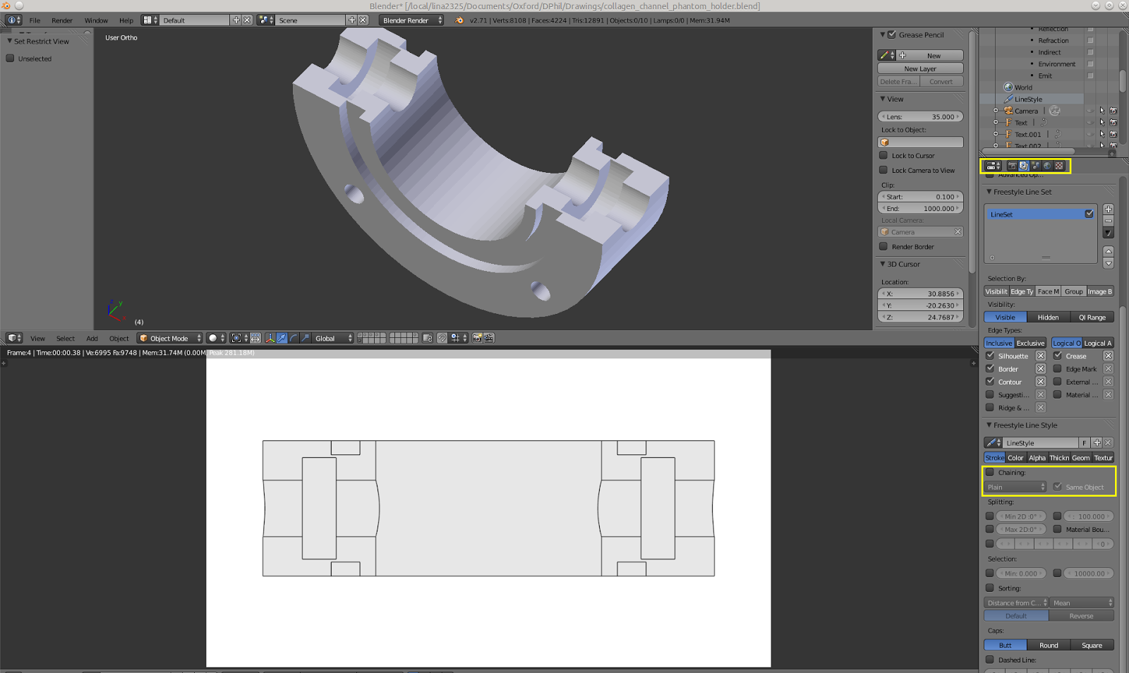Top is the model to be manufactured, bottom is a render of the model from the top in technical drawing style. In yellow are the necessary Free Style settings.

To achieve this look, you need to first set the camera to Orthographic mode, then enable Freestyle rendering in the render tab.

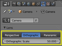In orthographic mode moving the camera towards or away from the object has no effect on its size. Orthographic Scale is what you need to change to "zoom" in and out.

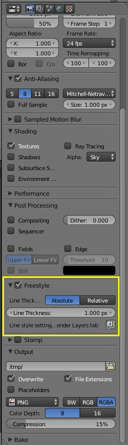Freestyle rendering is needed.

Lastly, it is necessary to use a shadeless white material since we don't want lighting of any kind.

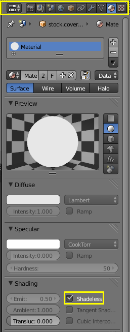A white shadeless material removes the need for lighting, and thus eliminates shading in the resulting render.

Internal Edges

It is possible to make internal edges, such as the edge of a channel, show up in the render. This is done by changing the Visibility setting in the Freestyle Render Layer settings.

When rendering internal edges, sometimes undesirable edges will show up. These can be convinced to go away by experimenting with the Edge Type checkboxes.

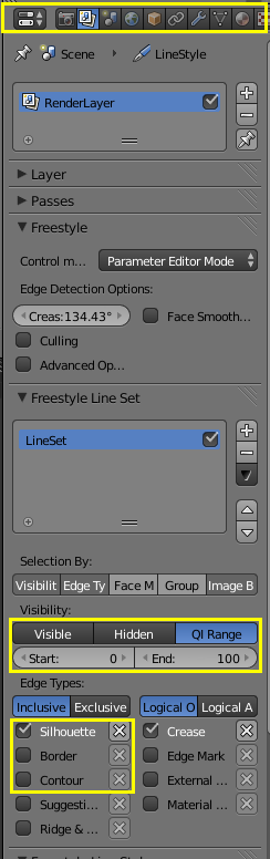QI range allows rendering of internal edges, while Edge Types allows elimination of undesirable internal edges.

Examples

Missing Features

Missing is the ability to add dimensions, that is something I haven't found a nice way of doing in blender, so for now it is added in post using Inkscape, or just by drawing on the printout.

Cheers,
Steve

Further Adventures in Python Optimisation

Previously we found that PyPy achieves the best performance gain, executing fieldfunc_py in ~6 us. At the end of that article, I mentioned that the C implementation is up to 50x faster, managing the same calculation in ~0.12 us.

The naive conclusion is that the best thing is to simply call the C function to do the heavy lifting, achieving performance somewhere between PyPy and C. But nothing in life is easy...

Naive C Interfacing

The C code in the previous article was compiled using

gcc -O -shared -o c_fieldfunc.so -fPIC c_fieldfunc.c

The MagnetElement class was then amended to use the C function whenever possible:

class MagnetElement(object):
  def __init__(self, position, size, magnetisation, fieldcalcfunc=fieldfunc_fast_py):
    """ 
    position, and magnetisation are all expected to be numpy arrays of 3
    elements each.

    size is a single number, implying all elements are square
    """

    self.position = position
    self.size = size
    self.magnetisation = magnetisation
    self.moment = magnetisation * size * size * size
    self._fieldcalcfunc = fieldcalcfunc

    try:
      import ctypes
      cmodule = ctypes.cdll.LoadLibrary('c_fieldfunc.so')
      self._fieldcalcfunc = cmodule.fieldfunc
      self.fieldAt = self._cfieldAt
    except OSError, ex: 
      pass

  def _cfieldAt(self, p): 
    import ctypes
    def voidp(x):
      return ctypes.c_void_p(x.ctypes.data)
    field = np.array([0,0,0], np.double)
    self._fieldcalcfunc(voidp(p),
                        voidp(self.position),
                        voidp(self.moment),
                        voidp(field))
    return field

  def fieldAt(self, p): 
    """ 
    p is expected to be a numpy array of 3
    """
    return self._fieldcalcfunc(p, self.position, self.moment)

This however yielded a per-run time of ~28 us!! So clearly there is significant cost in interfacing. The most obvious of these is creating a new np.array each time, and defining and calling voidp.

A Better C Interface

Below is an improved version:

class MagnetElement(object):
  def __init__(self, position, size, magnetisation, fieldcalcfunc=fieldfunc_fast_py):
    """ 
    position, and magnetisation are all expected to be numpy arrays of 3
    elements each.

    size is a single number, implying all elements are square
    """

    self.position = position
    self.size = size
    self.magnetisation = magnetisation
    self.moment = magnetisation * size * size * size
    self._fieldcalcfunc = fieldcalcfunc

    try:
      import ctypes
      cmodule = ctypes.cdll.LoadLibrary('c_fieldfunc.so')
      self._fieldcalcfunc = cmodule.fieldfunc
      self.fieldAt = self._cfieldAt
      self._field = np.array([0,0,0], np.double)

      def voidp(x):
        return ctypes.c_void_p(x.ctypes.data)
      self._position_p = voidp(self.position)
      self._moment_p = voidp(self.moment)
      self._field_p = voidp(self._field)
    except OSError, ex: 
      pass

  def _cfieldAt(self, p): 
    import ctypes
    self._fieldcalcfunc(ctypes.c_void_p(p.ctypes.data),
                        self._position_p,
                        self._moment_p,
                        self._field_p)
    return self._field

  def fieldAt(self, p):
    """
    p is expected to be a numpy array of 3
    """
    return self._fieldcalcfunc(p, self.position, self.moment)

Now we are down to ~7 us, which is about what PyPy gave us. We are still slower, and more effort is involved compared to the installing PyPy + numpy. That said, this method has the advantage that it is compatible with existing Python and numpy installations, and can be used to optimise python code that uses parts of numpy that are not yet implemented in PyPy.

Summary

• C interfacing needs to be done carefully to gain maximum benefit
• Not quite as easy as using PyPy, but more compatible

Addendum

While we achieved performance similar to PyPy using C interfacing in this one function, PyPy is going to give faster performance across the entire program, while Python+C will only speed up this one function. In my particular case, Python+C is over all ~2x as slow as PyPy.

Cheers,
Steve

Adventures in Python Optimisation

Recently I found myself looking at the following piece of code and trying to optimise it:

from __future__ import division

import numpy as np

MagneticPermeability = 4*np.pi*1e-7
MagneticPermeabilityOver4Pi = MagneticPermeability / (4*np.pi)

def fieldfunc_py(p, q, moment):
  r = p - q 
  rmag = np.sqrt(r.dot(r))

  rdash3 = rmag**3
  rdash5 = rmag**5

  rminus5term = r * moment.dot(r) * 3 / rdash5
  rminus3term = moment / rdash3

  field = (rminus5term - rminus3term) * MagneticPermeabilityOver4Pi
  return field

This, I have been told, computes the field at p due to a magnetic di-pole at q.

To profile this code I wrote the following function:

def profile(fieldfunc, dtype=np.double):
  def V(*args):
    return np.array(args, dtype)

  q = V(0, 0, 0)
  moment = V(1, 0, 0)
  p = V(10,10,10)

  def f():
    fieldfunc(p, q, moment)

  # force the JIT or whatever to run
  f()

  from timeit import Timer
  t = Timer(f)
  runs = 100000
  print fieldfunc.__name__,'per run', t.timeit(number=runs)*1e6/runs, 'us'

This yields a per-run time of ~22 us.

Optimise Python/Numpy

The first optimisation then is to write a better optimised version:

def fieldfunc_fast_py(p, q, moment):
  r = p - q
  rmag2 = np.dot(r, r)

  rdash3 = rmag2**1.5
  rdash5 = rmag2**2.5

  rminus5term = r * np.dot(moment, r) * 3 / rdash5
  rminus3term = moment / rdash3

  field = (rminus5term - rminus3term) * MagneticPermeabilityOver4Pi
  return field

The main difference is using np.dot() and avoiding np.sqrt(). Using ** is faster than using square root and multiplication. These changes gets us down to ~18 us or so, so slight improvement.

numba

Numba offers JIT compilation of python into native code, and is pretty easy to use and compatible with numpy. To use it the profile function was called as:

profile(jit(fieldfunc_py))
profile(jit(fieldfunc_fast_py))

Using jit without type arguments causes numba to infer the type. This yields per-run time of ~22 us for fieldfunc_py and ~18 us for fieldfunc_fast_py. There is no noticable speed up, in fact per-run times increased slightly. This is possibly due to the fact that the code is already pretty well optimised, and the extra overhead of interfacing between compiled code and the python runtime.

PyPy

PyPy is an altnerative implementation of Python that also uses JIT, but does it for the entire program. It is a little harder to use because it needs its own version of numpy, which is only partially implemented. For our needs this will suffice.

With PyPy, we see significant improvement. fieldfunc_py's per-run time went down to ~6 us, and fieldfunc_fast_py's per-run time went down to ~6 us also. This is a huge improvement.

Data Type Matters

The diligent reader may have noticed that profile accepts dtype as a keyword arguments. This was used to test the effects of using np.float32 vs np.float64. The following code was written:

for dtype in np.float32, np.float64:
  print 'With', dtype
  profile(fieldfunc_py, dtype)
  profile(fieldfunc_fast_py, dtype)

  try:
    from numba import jit
    print '==> Using numba jit'
    profile(jit(fieldfunc_py))
    profile(jit(fieldfunc_fast_py))
  except:
    pass

This yielded the following output using CPython:

With <type 'numpy.float32'>
fieldfunc_py per run 30.8365797997 us
fieldfunc_fast_py per run 27.7728509903 us
==> Using numba jit
fieldfunc_py per run 22.2719597816 us
fieldfunc_fast_py per run 18.1778311729 us

With <type 'numpy.float64'>
fieldfunc_py per run 21.8909192085 us
fieldfunc_fast_py per run 17.5257897377 us
==> Using numba jit
fieldfunc_py per run 22.4718093872 us
fieldfunc_fast_py per run 18.2463383675 us

Choice of data type has a significant effect, and it counter-intuitive: the larger data type is faster. Interestingly the same isn't true for PyPy, which outputted:

With <type 'numpy.float32'>
fieldfunc_py per run 6.29536867142 us
fieldfunc_fast_py per run 6.067070961 us

With <type 'numpy.float64'>
fieldfunc_py per run 6.28163099289 us
fieldfunc_fast_py per run 6.17563962936 us

Which is essentially the same.

How Fast Can It Be Done?

The final question is, how fast can this be done? Here is a naive C implementation:

#include <math.h>
#include <stdio.h>

typedef double dtype;

dtype vdot(dtype *u, dtype *v) {
  return u[0]*v[0] + u[1]*v[1] + u[2]*v[2];
}

/**
 * Computes w=u+v
 */
void vadd(dtype *u, dtype *v, dtype *w) {
  w[0] = u[0] + v[0];
  w[1] = u[1] + v[1];
  w[2] = u[2] + v[2];
}

/**
 * Computes w=u-v
 */
void vsub(dtype *u, dtype *v, dtype *w) {
  w[0] = u[0] - v[0];
  w[1] = u[1] - v[1];
  w[2] = u[2] - v[2];
}
/**
 * Computes w = x*u, returns w
 */ 
void vmult(dtype x, dtype *u, dtype *w) {
  w[0] = x*u[0];
  w[1] = x*u[1];
  w[2] = x*u[2];
}

#define MagneticPermeability          (4*M_PI*1e-7f)
#define MagneticPermeabilityOver4Pi   (MagneticPermeability/(4*M_PI))

void vprint(dtype *v) {
  printf("(%e, %e, %e)\n", v[0], v[1], v[2]);
}

void fieldfunc(dtype *p, dtype *q, dtype *moment, dtype *out) {
  dtype r[3];
  vsub(p, q, r);
  dtype rmag2 = vdot(r,r);

  dtype rdash3 = pow(rmag2, 1.5);
  dtype rdash5 = pow(rmag2, 2.5);


  dtype t5[3];
  vmult(vdot(moment, r), r, t5);
  vmult(3/rdash5, t5, t5);

  dtype t3[3];
  vmult(1/rdash3, moment, t3);

  vsub(t5, t3, out);
  vmult(MagneticPermeabilityOver4Pi, out, out);
}

int main(int argc, char **argv) {
  dtype q[] = {0, 0, 0};
  dtype p[] = {10, 10, 10};
  dtype moment[] = {1, 0, 0};
  dtype field[3];

  fieldfunc(p, q, moment, field);
  vprint(field);

  int x;
  for (x = 0; x < 1000000; ++x) {
    fieldfunc(p, q, moment, field);
  }

  return 0;
}

timing was done as follows:

$ gcc -o c_bench c_bench.c -lm && time ./c_bench 
(0.000000e+00, 1.924501e-11, 1.924501e-11)

real    0m0.116s
user    0m0.114s
sys     0m0.001s

Because we do 1 million iterations, per-run time is ~0.12 us, or around 50 times faster.

Summary

• Most gain/effort comes from using PyPy
• In this particular case, numba did not yield signficant speed up
• C is still much faster

Cheers,
Steve

Play Child of Light in English on PS Vita

If you want to play Child of Light on PS Vita, you will not only need to download the online update, you will also need to set your system language to English (US). If you have it set as English (UK) then you will continue seeing the game in Japanese.

I know right?

From Lyx/Latex to Word

This is sort of a placeholder post. Busy meeting a deadline, but this should help future Steve and anyone else when you need to turn your Lyx document into a Word document while keeping the format mostly sane. Broken, but sane.

1. Export as Latex (plain).
   
2. Run
   • latex <name of tex file, with or without extension>


3. Run
   • bibtex <filename>


4. Run
   • latex <filename>


5. Run
   • latex <filename>


6. Try to run
   • htlatex <filename> "html,0,charset=utf-8" "" -dhtml/
     • html: format to output
     • 0: normally chapters go into their own page, putting 0 here forces everything into a single page
     • charset=utf-8: let us be civilised
     • -dhtml/: puts the output files in a html sub-directory. Note that you can't have a space between -d and the html/


7. If the above fails with something like 'illegal storage address', and you get a warning about text4ht.env not been found, then you need to find where it is in your TeX installation, and:
   • export TEX4HTENV and try again
   • Copy text4ht.env into your working directory
     • This approach also lets you affect locally some export parameters. More on this later...


8. Open the html to verify correctness. You might object to the poor graphics quality. In this case copy text4ht.env into the working directory if you haven't done so, and then modify it so it uses a high density when converting images.
   
   • See this tex.stackexchange.com answer for more details
   • In my case, since dvipng was been used, I replaced all instances of
     • -D 96
   • with
     • -D 300


9. It also helps if you
   
   • strip away html comments
     • These look like <!-- xxx -->
   • centre aligned image divs
   • remove <hr/> instances


10. These changes will make the import into Libre/OpenOffice go easier


11. Open the html file in Libre/OpenOffice


12. File > Export > ODT


13. Close html file


14. Open exported ODT


15. Edit > Links


16. Select all links


17. Break Links


18. Verify that the ODT file is now much larger!


19. File > Save As > Word 97 (doc)

Phew! To help future visitors, a simple python script to fix up the html as I have described is included at the end of this post. You will need lxml and cssselector installed. Cheers, Steve

#!/usr/bin/env python

from lxml.html import parse, HtmlComment
from lxml import etree

def main(*args):
  if len(args) == 0:
    return 1

  doc = parse(args[0]).getroot()

  body = doc.cssselect('body')[0]

  # replace <hr/> with <br/> to make doc conversion easier
  for hr in body.cssselect('hr'):
    p = hr.getparent()
    p.remove(hr)

    br = etree.Element('br')
    p.append(br)

  # remove comments because for some reason libreoffice opens up 
  # html comments as document comments, slowing things down
  for node in doc.getiterator():
    if isinstance(node, HtmlComment):
      node.getparent().remove(node)

  # centre align all figures
  for div in doc.cssselect('div.figure'):
    div.attrib['style']='text-align:center'

  print etree.tostring(doc, method='html', encoding='utf-8')
if __name__ == '__main__':
  import sys
  sys.exit(main(*sys.argv[1:]))

Reading Metadata Out of Nikon NIS Elements Generated TIFFs

Fluorescence image of 
cavitation effects,visualised 
using FITC-Dextran.

If, like me, you use Nikon's NIS Elements to do fluorescence imaging, you would have also noticed that nothing other than NIS Elements can read the metadata that is saved with TIFFs. ImageJ can't read it, the GIMP can't read it, tiffinfo can't read it. This means the only way to recover that metadata, which contains important things like exposure time and pixel size is to open the image in NIS Elements.

This sucks, because NIS Elements isn't exactly easily or widely available, and NIS Elements Viewer doesn't help either - it only opens ND3 files.

Fret not, however. The metadata isn't encoded in any particularly nasty way, and with a little exploration I was able to put together a small python script which will dump out all the relevant information.

Hope this helps someone. It would be nice if Nikon used the standard TIFF tags instead of putting everything in their own tags.

Cheers,
Steve

Go Away AVN

So it turns out that if you google vaccination on google.com.au, Australian Vaccination Network (AVN) comes up as the second result, right after wikipedia.

Search results from google.com.au for
"vaccination" as of 20th of May 2013

As some of you may know, AVN is an anti-vaccination organisation, part of the anti-vaccination movement, whose core beliefs rests on a retracted paper published by a doctor who was struck off the UK medical register after been found guilty of unprofessional and unethical conduct.

Vaccination is a corner stone of public health policy, and the only means of protection for the most vulnerable amongst us who are unable to receive vaccinations. Through vaccination smallpox was eradicated in 1979, and no child was ever again killed or maimed by it.

A child with smallpox

Due to the efforts of groups like the AVN however, there has been recent decline in the number of children receiving vaccinations against common childhood whooping cough, leading an outbreak of whooping cough in Queensland, and sadly, the death of several infants.

While the Australian Government is taken action against the AVN, the fact it has such a prominent position in Google's search results is undermining the overall effort. Thankfully this is something you and I can do something about, and that is what this blog post is for: part of an effort to increase the PageRank of legitimate sources of vaccination like

• http://www.vaccination.org.au/ 
• http://www.immunise.health.gov.au/

If you have a blog, make a post like this one, google vaccination on google.com.au and click on every result that is NOT AVN.

Cheers,
Steve